Space-Vector PWM Study Notes – Understanding Fundamental Concepts

Space-vector PWM and associate concepts and techniques such as abc-dq transformation, zero-vector-injection and so on are very abstract to learn. I recently started to review them for a 3-phase ac-dc project. While they are commonly used, I was a little frustrated that it’s hard to find a place online that connects dots among these concepts, moreover there are lots of incorrect materials that either misdefined concepts, or had wrong derivation. Some tutorials have animations that can help visualize the concepts, yet they didn’t provide enough quantitative explanation, while others focus too much on the math and distant from the physical meaning. As such I decided to synthesize and reflect on the process of understanding these topics with some notes of my own.

DISCLAIMER: this article is more for myself to keep track of my thoughts and to clarify some concepts of SVPWM that I have struggled with. While I tried to organize the material in a logical sense for better understanding, it is NOT intended to teach SVPWM from zero knowledge. Moreover, the derivations and conclusions are directly from the fundamental concept of SVPWM, so I didn’t cite any reference. If you found anything that might have been published, please let me know so I can cite properly.

1. The initial misunderstanding of Space Vector v.s. Voltage Phasors

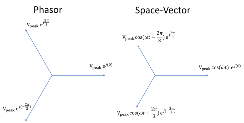
When I first learned about using space vector to represent 3-phase voltages, I found myself often confused between space vector and phasor vector that I learned very early in undergrad EE classes.

In time domain, the three-phase voltages are

$v_{an} = V_\text{peak}\cos(\omega_L t),v_{bn} = V_\text{peak}\cos(\omega_L t - \frac{2\pi}{3}),v_{cn} = V_\text{peak}\cos(\omega_L t + \frac{2\pi}{3})$

In the phasor domain, while the three phase voltages are also represented by three vectors that are separated with $\frac{2\pi}{3}$ , the magnitude of the vectors do not change, as it is equal to $V_\text{peak}$ . For the space vector, the magnitude of the vectors change with the time-domain voltages as shown above, and they are $\frac{2\pi}{3}$ apart in phase. I was quite confused by this representation first because why the length of the vectors is also related to the phase angle $\frac{2\pi}{3}$ , while they are already $\frac{2\pi}{3}$ apart in the phase?.

Three-phase voltage representation in steady-state phasor domain and space-vector domain

Then I realized that the physical meaning is much more clear in a three-phase electric motor layout. The $\frac{2\pi}{3}$ in the space vector space (or abc space) is the reflection of the physical layout of the three-phase winding, and the magnitude of the three-phase voltages change in time domain. Thus, the phase angles of the three vectors are actually the physical layout angle of the winding.

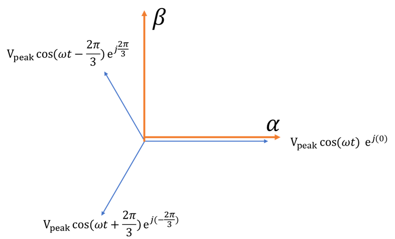
2. Adding three-phase vectors in the Space-Vector plane with Clarke Transformation

Since now it’s clear that the three-phase vectors in their 2-d space are $\frac{2\pi}{3}$ apart and with time-varying magnitudes, we can define the x-axis and y-axis of the existing 2-d space of the three vectors. And this 2-d space is referred as $\alpha-\beta$ space, with $\alpha$ being x-axis (0 degree), and $\beta$ being y-axis (90 degree)

Three-phase voltage representation in alpha-beta domain

Essentially, the aforementioned vector representation is in polar coordinates, with magnitude and phase being the two coordinates in the plane to represent one vector. In algebra, there are two ways to compute the addition of vectors:1. solve the geometry, or compute using (x,y) coordinates. Computing using (x,y) is usually more convenient to get the results, yet it is also not as intuitive as graphical representation. The famous $abc-\alpha \beta$ transformation (Clarke Transformation) is the method to convert the polar information of the vectors to (x,y), or $\alpha \beta$ values. However, there is a scalar of $\frac{2}{3}$ that needs to be noticed. If we simply project the three voltage vectors onto $\alpha\beta$ axises, we will get

$\begin{bmatrix}V_\text{$\alpha$}\\V_\text{$\beta$}\end{bmatrix}=\begin{bmatrix}\cos (0) & \cos (2\pi/3) & \cos (-2\pi/3)\\\sin (0) & \sin (2\pi/3) & \sin (-2\pi/3)\\\end{bmatrix}\begin{bmatrix}V_{an}(t)\\V_{bn}(t)\\V_{cn}(t)\end{bmatrix}$

The results are :

$\begin{bmatrix}V_\text{$\alpha$}\\V_\text{$\beta$}\end{bmatrix}=\frac{3}{2}\begin{bmatrix}V_\text{peak}\cos(\omega_L t)\\V_\text{peak}\sin(\omega_L t)\end{bmatrix}$

This means that the resultant summed vector has a magnitude that is 1.5 times of the line voltage magnitude $V_\text{peak}$ . This is a common mistake or inconsistency among different online tutorials and videos. For instance, if in a system controller, the reference of the final summed voltage is $v_\text{ref} = V_\text{ref}\cos(\omega t)$ , the relation between line-voltage magnitude and reference voltage is $V_\text{ref} = 1.5V_\text{peak}$ . In some sources, you will find this relation is used in all of the derivations. Yet, the formal CLARKE TRANSFORMATION has a 2/3 scalar in front of the matrix as

$\begin{bmatrix}V_\text{$\alpha$}\\V_\text{$\beta$}\end{bmatrix}=\frac{2}{3}\begin{bmatrix}\cos (0) & \cos (2\pi/3) & \cos (-2\pi/3)\\\sin (0) & \sin (2\pi/3) & \sin (-2\pi/3)\\\end{bmatrix}\begin{bmatrix}V_{an}(t)\\V_{bn}(t)\\V_{cn}(t)\end{bmatrix}$

The updated $\alpha \beta$ voltages are:

$\begin{bmatrix}V_\text{$\alpha$}\\V_\text{$\beta$}\end{bmatrix}=\begin{bmatrix}V_\text{peak}\cos(\omega_L t)\\V_\text{peak}\sin(\omega_L t)\end{bmatrix}$

From basic algebra, we know that the updated summed vector rotates in a circle, with radius of $V_\text{peak}$ and angular speed of $\omega_L$ .
Seeing the circle reinforced the physical meaning of a rotating vector. The reason that the 3-phase ac motor rotates is because of this rotating voltage vector, which generates a rotating electromagnetic field vector.

Anyways, the main takeaway is that it is recommended to use

$V_\text{ref} = V_\text{peak}$

for all the derivations, since most papers used results derived from this relation

3. Understanding the coded vector space of SVPWM

3.1 Space-vector PWM using 6-switch 2-level inverter: what is the vector of each switching state?

6-switch, 2-level (2-level each leg), 3-phase inverters are the most common 3-phase topology to apply space-vector PWM.

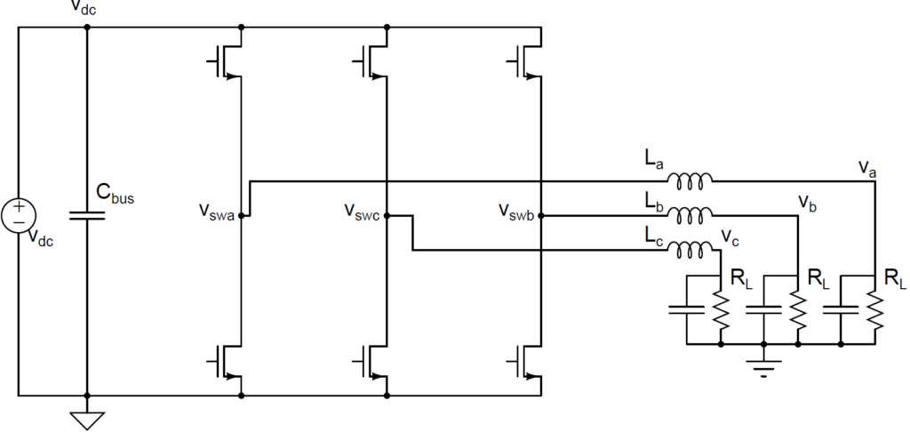
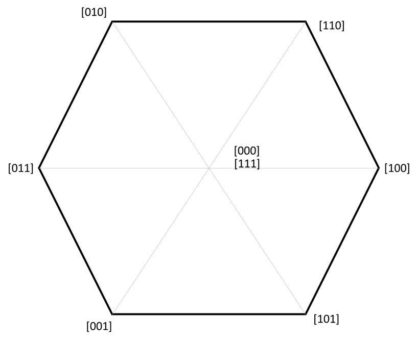
The convention is that since there are 6 switches and 3 phases, each phase is either 0 as low-side switch is on, and 1 as high-side switch is on. So the states of the switches can be represented as 3 bit binary code [Sa, Sb, Sc] = [100] [110]… and so on.

There are many tutorials that covers this process. Yet the first thing that took me a while to get was:

The vector length of each coded vector

For instance, [100] means the high side switch of phase A is on, and B and C are connected to the low-side. Note that the dc-bus negative common node is not the same as the ac neutral node. We can draw the equivalent circuit in [100] as below

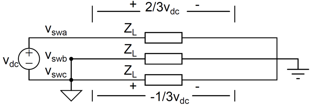
In a balanced 3-phase system, the impedance of each phase ZL is the same. With basic voltage divider rule we can find the values of three-phase line-neutral voltages are

$\begin{bmatrix}V_{an}(t)\\V_{bn}(t)\\V_{cn}(t)\end{bmatrix} = \begin{bmatrix}\frac{2}{3}V_{dc}\\\frac{-1}{3}V_{dc}\\\frac{-1}{3}V_{dc}\end{bmatrix}$

Using the Clarke Transformation, the vector in $\alpha-\beta$ coordinates can be found as

$V_{\alpha} = \frac{2}{3}(\frac{2}{3}V_{dc}+(-\frac{1}{2})\frac{-1}{3}V_{dc}+(-\frac{1}{2})\frac{-1}{3}V_{dc}) =\frac{2}{3}V_{dc} \\, V_{\beta} = 0$

The coded vectors [100] etc all have a length of 2/3 Vdc

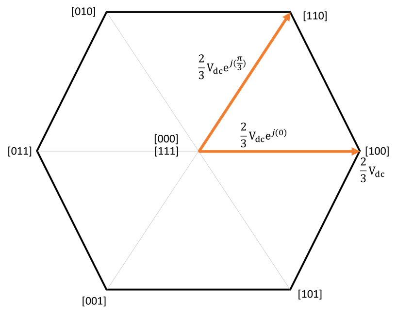
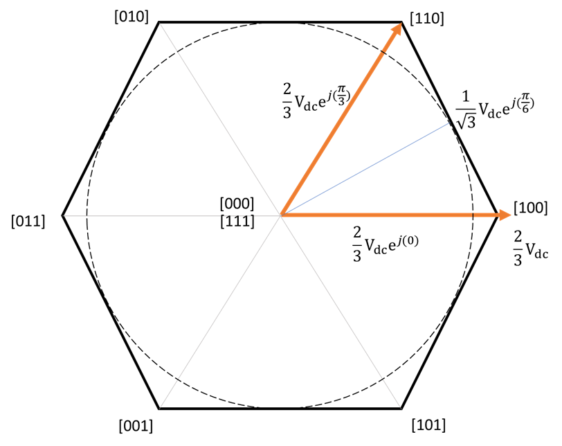
This means that the voltage vector encoded with [100] has length of $\frac{2}{3}V_{dc}$ and a phase of zero. Thus, in the common hexagon diagram of SVPWM, except for zero vector [000] and [111], the length of each coded voltage vector [110] [010] etc is $\frac{2}{3}V_{dc}$ , (not $V_{dc}$ as in some material)

3.2 Why the achievable voltage vector space is bounded by a hexagon not a circle with radius 2/3Vdc?

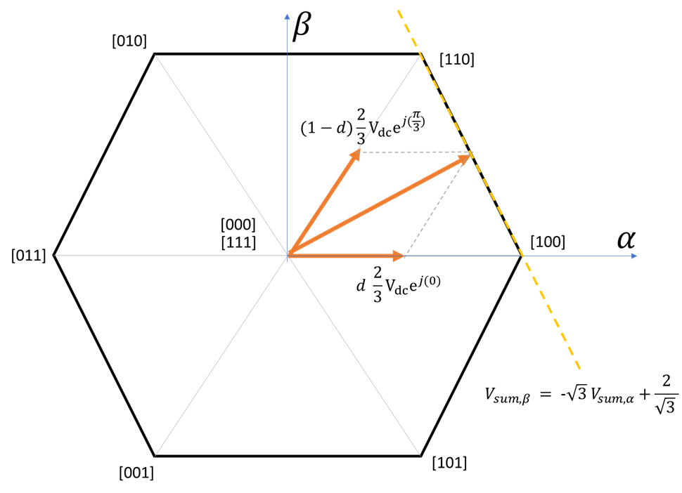
Once I derived the length of the coded vectors, I had a question that why the available vector space has a hexagon boundary, not a circle with $\frac{2}{3}V_{dc}$ radius. Most sources just default this fact, but this boundary can be derived using the average of the two available vectors. Since the principle of SVPWM is to create a time-averaged vector using the two adjacent available coded vectors, we can derive the expression of the achievable vector assuming no zero vector is in one switching cycle.

We start with the space between the vector [100] and [110]. Say that in one switching cycle, we spend a fraction of $d$ (duty ratio, 0 to 1) on [100] ( $(\frac{2}{3}V_{dc}, 0)$ in $\alpha-\beta$ ) and $(1-d)$ on [110] ( $(\frac{2}{3}V_{dc}\cos\frac{\pi}{3}, \frac{2}{3}V_{dc} \sin(\frac{\pi}{3})$ in $\alpha-\beta$ ), the resulted voltage vector in $\alpha-\beta$ coordinate is:

$\begin{bmatrix}V_\text{sum, $\alpha$}\\V_\text{sum, $\beta$}\end{bmatrix}=d\begin{bmatrix}\frac{2}{3}V_{dc} \\0 \\\end{bmatrix}+(1-d)\begin{bmatrix}\frac{2}{3}V_{dc} \cos(\frac{\pi}{3}) \\\frac{2}{3}V_{dc} \sin(\frac{\pi}{3}) \\\end{bmatrix}=V_{dc}\begin{bmatrix}\frac{1+d}{3} \\\frac{(1-d)}{\sqrt{3}} \\\end{bmatrix}$

If we plot the coordinates with d from 0 to 1, we can get the hexagon boundary between [100] and [110] as a straight line:

$V_\text{sum, $\beta$} = -\sqrt{3} V_\text{sum, $\alpha$} + \frac{2}{\sqrt{3}}$

The yellow dashed line is the derived boundary of the SVPWM

3.3 What is the maximum achievable line-neutral voltage?

From Clarke transformation, we know that the final summed vector is rotating with radius $V_\text{peak}$ . Basically, this question is equivalent to, how high $V_\text{peak}$ can be?

The explanation was to draw a circle inside the hexagon that is tangent to the hexagon, with that we can find the radius of the circle to be $\frac{\sqrt{3}}{2}* \frac{2V_{dc}}{3} = \frac{V_{dc}}{\sqrt{3}}$ , which is $V_\text{peak}$ . That is, the maximum line-neutral voltage with $V_{dc}$ is $\frac{V_{dc}}{\sqrt{3}}$

Blogs