Now the basic concepts of SVPWM are discussed, the next step is to generate the desired three-phase voltage with SVPWM.
1. Generating  by adding two average vectors along coded phases
First, as discussed in previous post on fundamental concepts of SVPWM, the reference rotating vector you want to generate has a magnitude that is equal to the peak line-neutral voltage. As such, we define the reference voltage as
![\[ v_\text{ref} = V_\text{ref}\cos(\omega_L t) = V_\text{peak}\cos(\omega_L t) \]](https://www.liaozitao.org/blog/wp-content/ql-cache/quicklatex.com-ebccc3f09be68421ce9d8c47a1160b2e_l3.png "Rendered by QuickLaTeX.com")
Or exponential form 
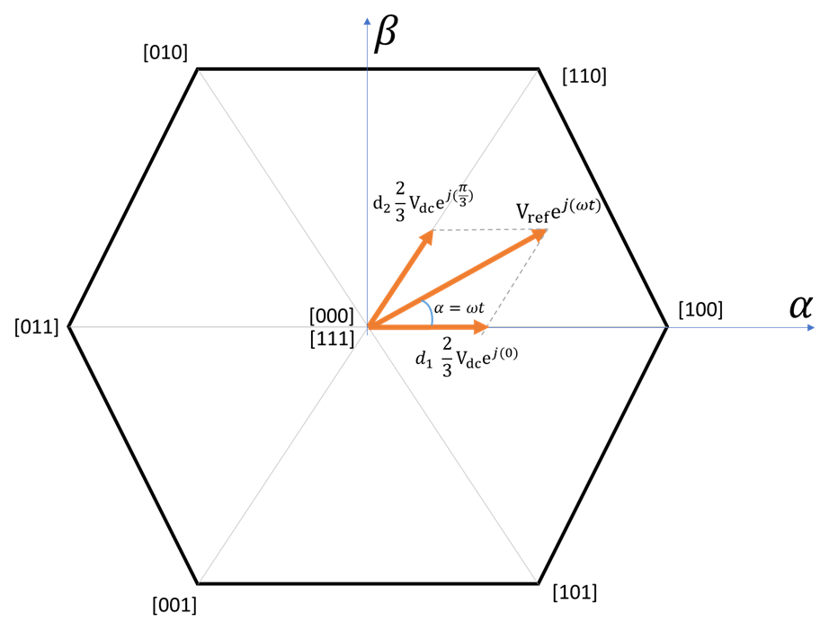
In 0 to  region, the final vector is the sum of the average vectors on [100] and [110]. That is, in one switching cycle, the time that is spent in the direction of vector [100] is
  , (where
  is the duty ratio,
  is the switching period) and time in the direction of [110] is
The average vector in the phase of [100] is thus  and
and  in the phase of [110]. To write more formally in the format of vector algebra:
![\[\vec{V_{ref}} = d_1\vec{V_{[100]}} + d_2\vec{V_{[110]}} \]](https://www.liaozitao.org/blog/wp-content/ql-cache/quicklatex.com-f3f5a5ebffbac6010b96b78485c11916_l3.png "Rendered by QuickLaTeX.com")
Thus we need to solve  so we can generate the correct average vectors.
2. Different ways to solve d1 and d2
2.1 Solve the triangular geometry
The most intuitive way is to solve the length of the vectors so we can calculate the portion of the vector on the coded vector [100] and [110] as shown below.
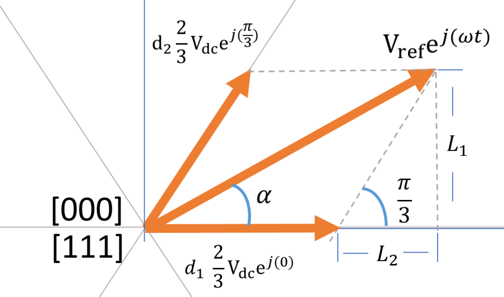
To solve for the length of  and
and  , there are two auxiliary lines with
  and
and  lengths we can use as shown above
The length of can be obtained by subtracting from  , and the length of
  can be obtained with
  as they are in the same triangle. We can get the following equations to solve:
![\[ L_1 = V_{ref}\sin(\alpha) = d_2\frac{2V_{dc}}{3}\sin(\frac{\pi}{3}) \]](https://www.liaozitao.org/blog/wp-content/ql-cache/quicklatex.com-926ed1d093c128c2265785d62d3cf7bb_l3.png "Rendered by QuickLaTeX.com")
![\[ L_2 = d_2\frac{2V_{dc}}{3} \cos(\frac{\pi}{3}) \]](https://www.liaozitao.org/blog/wp-content/ql-cache/quicklatex.com-96d1b7bf1086cdd57fc73b85c125a6bc_l3.png "Rendered by QuickLaTeX.com")
![\[ V_{ref}\cos(\alpha) = d_1\frac{2V_{dc}}{3} + L_2 \]](https://www.liaozitao.org/blog/wp-content/ql-cache/quicklatex.com-60465fd6e9f710a4820908195a5f2d93_l3.png "Rendered by QuickLaTeX.com")
using the first equation we can easily solve for  as
as
![\[ d_2 = \frac{V_{ref}\sin(\alpha)}{\frac{2V_{dc}}{3}\sin(\frac{\pi}{3})} = \frac{\sqrt{3}V_{ref}\sin(\alpha)}{V_{dc}} = \sqrt{3}m\sin(\alpha) \]](https://www.liaozitao.org/blog/wp-content/ql-cache/quicklatex.com-3545f8ad4c8e4cc726d3473a337442e8_l3.png "Rendered by QuickLaTeX.com")
In some materials, they define the modulation index  . Once is solved, we can get the vector length on [100]
![\[ d_1\frac{2V_{dc}}{3} = V_{ref}\cos(\alpha) - L_2 = V_{ref}\cos(\alpha) - \frac{V_{ref}\sin(\alpha)\cos(\frac{\pi}{3})}{\sin(\frac{\pi}{3})} = V_{ref}(\cos(\alpha)-\frac{\sin(\alpha)}{\sqrt{3}}) \]](https://www.liaozitao.org/blog/wp-content/ql-cache/quicklatex.com-dba02b8b85a8b0650d82002564d126a6_l3.png "Rendered by QuickLaTeX.com")
And can be solved as
![\[ d_1= V_{ref}\frac{2}{\sqrt{3}}\cos(\alpha+\frac{\pi}{6})\frac{3}{2V_{dc}} = \sqrt{3}\frac{V_{ref}}{V_{dc}}\cos(\alpha+\frac{\pi}{6}) = \sqrt{3}m\cos(\alpha+\frac{\pi}{6}) \]](https://www.liaozitao.org/blog/wp-content/ql-cache/quicklatex.com-17e55d2c5434e4bf3199f4f2c9f2a089_l3.png "Rendered by QuickLaTeX.com")
This is just one way to solve the geometry, you can draw different triangles to get the vector lengths.
2.2 Solve using  coordinates
Since vectors can be represented with coordinates, this problem can also be completely computed using linear algebra.
![\[ V_\text{peak}\begin{bmatrix} \cos(\alpha)\\\sin(\alpha) \end{bmatrix} = \frac{2V_{dc}}{3} d_1 \begin{bmatrix}\cos(0)\\ \sin(0)\end{bmatrix} + \frac{2V_{dc}}{3} d_2\begin{bmatrix}\cos(\frac{\pi}{3})\\ \sin(\frac{\pi}{3})\end{bmatrix} \]](https://www.liaozitao.org/blog/wp-content/ql-cache/quicklatex.com-ce1826e0d35b378395c33d261b75c936_l3.png "Rendered by QuickLaTeX.com")
![\[ V_\text{peak}\begin{bmatrix} \cos(\alpha)\\\sin(\alpha) \end{bmatrix} = \frac{2V_{dc}}{3}\begin{bmatrix}\cos(0)& \cos(\frac{\pi}{3})\\ \sin(0) &\sin(\frac{\pi}{3})\end{bmatrix} \begin{bmatrix} d_1\\d_2\end{bmatrix} \]](https://www.liaozitao.org/blog/wp-content/ql-cache/quicklatex.com-1ed1040a5426fcd2fb54f665285e33ff_l3.png "Rendered by QuickLaTeX.com")
And can be solved by inverting the matrices. Since the results are the same, I won’t expand the derivation.